How does the order we access the elements of a 2D array affects program performance? In particular, does it make any difference to access the elements in row-major vs column-major order?
In this post, we’ll analyze a program manipulating 2D arrays. Both row-major and column-major reference patterns will be studied. The performance will be assessed using perf_events. Finally, we will explain the results in terms of program locality and memory caching. These results can be generalized to other multidimensional arrays besides 2D.
The example program will be written in C.
Analyzing the difference in reference order: row-major vs column-major
Given an array A[N][M], we’ll analyze these two different reference patterns:
for (i = 0; i < N; i++)
  for (j = 0; j < M; j++)
    process A[i][j]
1. row-major
for (j = 0; j < M; j++)
  for (i = 0; j < N; i++)
    process A[i][j]
2. column-major
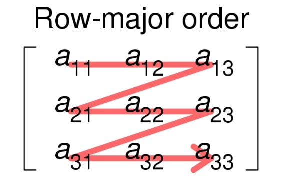
The first variation accesses array elements in the order A[0][0], A[0][1], A[0][2], …, A[0][M], A[1][0], A[1][1], … and so on. See that all of the elements in the first row are accessed first, then those in the second row, and so on. This is known as row-major.

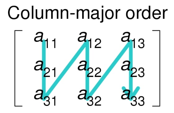
The second example accesses the elements in the order A[0][0], A[1][0], A[2][0], …, A[N][0], A[0][1], A[1][1], … and so on. We get all of the elements of the first column first, then those of the second column, and so on. This is known as column-major.

Evaluated program
To determine the effect on performance, we’ll analyze a simple program that performs 2 operations on array A[N][M]:
- Fill all of the elements in the array with a value.
- Sum all of the elements in the array.
We’ll measure the performance executing those two actions with different array dimensions. For every case, the different reference patterns will be evaluated separately.
| rows (N) | columns (M) |
| 1814400 | 2 |
| 1209600 | 3 |
| 907200 | 4 |
| 725760 | 5 |
| 604800 | 6 |
| 518400 | 7 |
| 453600 | 8 |
| 403200 | 9 |
| 362880 | 10 |
See that the total number of elements (N x M) is always 10! (3628800). This way, for every variation, we’re performing the same number of operations.
Filling the array
The first operation consists of initializing the array data. See that the array contains elements of data-type long.
void inita(int rows, int cols, long data[][cols]) {
  for (int i = 0; i < rows; i++)
    for (int j = 0; j < cols; j++)
      data[i][j] = 1;
}
We’re completely filling data with value 1. The code snippet above is the row-major variant. The column-major one is similar, except that the order of the for loops is swapped:
void initb(int rows, int cols, long data[][cols]) {
  for (int j = 0; j < cols; j++)
    for (int i = 0; i < rows; i++)
      data[i][j] = 1;
}
Getting the sum of all elements
The second operation will calculate the total sum of the elements in the array data.
void suma(int rows, int cols, long data[][cols], long *ptotal) {
  long total = 0;
  for (int i = 0; i < rows; i++)
    for (int j = 0; j < cols; j++)
      total += data[i][j];
  *ptotal = total;
}
Again, the column-major variant is the same, with the for loops order inverted.
void sumb(int rows, int cols, long data[][cols], long *ptotal) {
  long total = 0;
  for (int j = 0; j < cols; j++)
    for (int i = 0; i < rows; i++)
      total += data[i][j];
  *ptotal = total;
}
Main routine
These two operations are performed after allocating the array in memory using malloc.
#define SIZE 3628800

int main(int argc, char **argv) {
  int cols = atoi(*++argv);
  int rows = SIZE / cols;
  long total;
  long (*data)[cols] = malloc(sizeof(long[rows][cols]));
  inita(rows, cols, data);
  suma(rows, cols, data, &total);
  free(data);
  return 0;
}
The number of columns, cols, is passed as an argument to the program. Above, we show the code for row-major evaluation. The column-major version would use initb and sumb instead of inita and suma.
Measuring performance
Once we have the program (file sum.c), we evaluate its performance using the profiling Linux toolperf.
We compile the program with the -Og flag to avoid compiler optimizations that could modify the performance.
$ gcc -Og -o main sum.c
The performance can be evaluated using perf as follows:
$ perf stat -d --repeat 100 ./main 2 a

 Performance counter stats for './main 2 a' (100 runs):

             20,05 msec task-clock                #    0,983 CPUs utilized            ( +-  0,89% )
                 2      context-switches          #    0,106 K/sec                    ( +-  6,32% )
                 0      cpu-migrations            #    0,000 K/sec                    ( +-100,00% )
             7.138      page-faults               #    0,356 M/sec                    ( +-  0,00% )
        67.778.924      cycles                    #    3,381 GHz                      ( +-  0,12% )
        31.984.724      stalled-cycles-frontend   #   47,19% frontend cycles idle     ( +-  0,26% )
        23.448.897      stalled-cycles-backend    #   34,60% backend cycles idle      ( +-  0,34% )
       109.762.039      instructions              #    1,62  insn per cycle
                                                  #    0,29  stalled cycles per insn  ( +-  0,01% )
        22.636.470      branches                  # 1129,067 M/sec                    ( +-  0,01% )
            22.245      branch-misses             #    0,10% of all branches          ( +-  0,96% )
        11.031.695      L1-dcache-loads           #  550,242 M/sec                    ( +-  0,02% )
         1.098.152      L1-dcache-load-misses     #    9,95% of all L1-dcache hits    ( +-  0,12% )
           501.214      LLC-loads                 #   25,000 M/sec                    ( +-  0,34% )
   <not supported>      LLC-load-misses

          0,020403 +- 0,000184 seconds time elapsed  ( +-  0,90% )
The first argument, 2, is the number of columns. The complete program also accepts a second parameter,a or b, indicating whether the row-major or the column-major variant is executed. The results shown are for the average over 100 runs.
We can see that perf provides a wealth of information. From the actual cycles the processor takes to execute the program, to other low-level information, such as missed branches, and cache misses.
To analyze the performance, we’ll focus on three variables: cycles, L1-dcache-loads, and L1-dcache-load-misses. The latter two will be used to calculate the miss rate.
Performance results
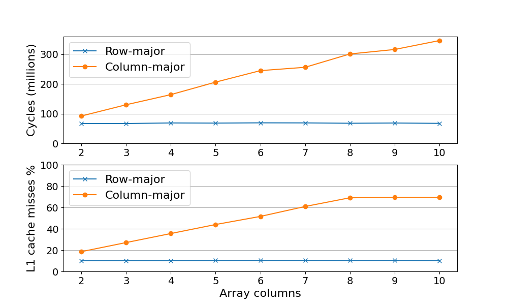
The same process was repeated using a variable number of columns (2 to 10) with row- and column-major programs. The results are summarized below.

The top graph shows the number of processor cycles that it takes to complete the program. See that while the row-major program completes using the same number of cycles (about 70K) regardless of the array dimensions, the column-major program increases the number of cycles with the number of columns.
This increase in cycles can be understood with the cache misses rate (bottom graph). This percentage is calculated as cache misses/ cache loads (more details in the next section). During cache misses, the processor needs to wait for the data to be loaded, which increases the cycle count. Again, the row-major program shows a constant trend (about 10% cache misses). For the column-major program, the percentage of cache misses increases with the number of columns in the array. It reaches a maximum at M=8 (about 70%) and then remains constant.
The effect of memory caching
Processors can execute operations extremely fast. To execute some operations, they need data. This data comes from the main memory (RAM) or the disk. These storage devices can transfer data to the processor at a very slow rate (for the processor). In order to bridge this gap, the processor includes low-capacity (between KB and a few MB), fast-access devices known as cache memories. They load information from the other slower devices for the processor to access them with lower access times.
This is how it works: the processor will request data (the array values) from the main memory. It will try to get it directly from the cache memories (cache load). Initially, they are all empty. In the absence of the required piece of data, we’ll have a cache miss. Then, the cache memories will load the requested information from the main memory. As it was mentioned, loading data from the main memory is slow and the processor will sit idle while it waits for the data to be loaded. That’s why we want to keep the cache misses to a minimum.
Data is loaded to the CPU cache from the main memory in blocks. For example, this demonstration used a processor with a cache block size of 64 bytes. For data type long, which has a size of 8 bytes, the same block can contain up to eight different elements. That means that whenever a block with long data is read from the main memory, 8 values are loaded to the cache.
Accessing data from nearby memory locations is known as spatial locality. If we access the data in the order it’s stored in the main memory (sequential access), we’ll make the best use of the fast access cache memories. In the context of our example program, after the initial cache miss, there are 7 more values loaded in the same cache block. If the next array references are to the elements contained in that block, the processor will be able to load them fast and the program performance will improve. We’ll have only 1 miss out of 8 loads. See that 1/8 corresponds to 12.5%, which is about the cache miss percentage of the row-major program!
On the other hand, accessing data non-sequentially is sub-optimal. In general, accessing data every k elements is called a stride-k access pattern. For example, a stride-2 access pattern would access elements i, i + 2, i + 4, etc in a linear array. Let’s take a stride-8 access pattern. If every block contains 8 elements, we’ll need one block for each array reference. This pattern leads to the highest miss rate.
Now that we know about caching, the key to explaining the performance results is to understand how data is stored in memory for a multidimensional array.
Array data storage in memory
All arrays store data in contiguous memory addresses. For a linear array, this is quite simple. If the first element is at address i, the second one is at i + 1, and so on.
Multidimensional arrays are actually the same. When we compile our program, all multidimensional arrays are “converted” to linear arrays. Programming languages such as C, store the memory elements in row-major order.
Row-major order is used in C/C++/Objective-C (for C-style arrays), PL/I, Pascal, Speakeasy, SAS, and Rasdaman.
Wikipedia
That means that when we access our data in row-major order, we’re actually accessing elements in the order they are stored in memory. We’re accessing elements sequentially.
On the other hand, accessing data in column-major order, when the data is actually stored in row-major order, is the same as accessing data in a stride-k access pattern, where k is the number of columns. This explains why the cache miss rate is greater for the column-major version of our program. And also why we reach a maximum miss rate at 8 columns. Since the cache block size is 64 bytes, each block contains 8 long data elements. Requesting data at a stride-8 or greater is the same as requesting a new block with every array reference.
However, referencing array elements in row-major order isn’t an absolute rule. Some programming languages store elements in column-major order. For those programming languages, the best approach is to reference arrays in column-major order.
Column-major order is used in Fortran, MATLAB, GNU Octave, S-Plus, R, Julia, and Scilab.
Wikipedia
Multidimensional arrays
While it’s a bit difficult to visualize how a multidimensional array (other than 2D) is transformed to a linear array in row-major order, there’s a simple rule that can be used to reference elements sequentially.
While referencing the elements as A[n0][n1]...[ni], the indices should vary faster as we move towards the right. That means ni is modified the fastest and n0 the slowest as we loop through the elements.