The Memory Mountain is a graphical representation of the read bandwidth (the rate data is read by a program in MB/s) in terms of the total data size processed and its access pattern. It provides great insight into the way CPU cache helps bridge the gap between the high-speed processor and the relatively slow access times of the main memory. It was introduced by Stricker and Gross, and I first read about it in Computer Systems: A Programmer’s Perspective (CS:APP).
In this post, we’ll generate a memory mountain with the diagnostic program provided by CS:APP and plot it using Python’s matplotlib. Then we’ll analyze it to gain some insight about the memory hierarchy. In particular, we’ll estimate the CPU cache sizes.
Measuring the memory read bandwidth
As it was mentioned, the program used to measure the read bandwidth is the one provided by CS:APP. You can get it from their website (file mountain.tar in the Chapter 6 section).
Data
The program allocates 128 MB of memory for an array of long elements (long is usually 8 bytes).
#define MAXELEMS (1 << 27)/sizeof(long)

long data[MAXELEMS];
It then proceeds to initialize the array with each element as data[i] = i.
for (int i = 0; i < n; i++)
  data[i] = i;
Testing memory access
The actual operation that is measured, is the test function. This function iterates over some elements of the array to calculate their total sum. In order to take advantage of modern processors parallelism, this operation is performed by 4 accumulators simultaneously.
int test(int elems, int stride) {
  ...
  for (long i = 0; i < elems; i += sx4) {
    acc0 = acc0 + data[i];
    acc1 = acc1 + data[i+stride];
    acc2 = acc2 + data[i+sx2];
    acc3 = acc3 + data[i+sx3];
   }
  ...
  return ((acc0 + acc1) + (acc2 + acc3));
}
A couple of parameters come into play here: the number of elements elems, and the stride.
The first one, elems, is derived from the portion of the array that is processed expressed by the variable size in bytes.
int elems = size / sizeof(long);
size values correspond to 16KB, 32 KB, 128 KB, 256 KB, 512 KB, 1 MB, 2 MB, 4 MB, … up to 128 MB.
The stride defines the access pattern. The simplest one is stride=1, which corresponds to sequential access: we access the array elements in the order i, i + 1, i + 2, etc. In general, a stride-k access pattern would access the array elements in the order: i, i + k, i + 2k, etc.
stride takes values between 1 and 15.
The other variables in the code snippet, sx2, sx3, and sx4, are just multiples of stride used to process the multiple sum accumulators (acc0 to acc3) in parallel.
Measuring performance
The fcyc2 function measures the CPU cycles it takes test to run. With this information, as well as the processor’s clock rate (obtained from /proc/cpuinfo, variable Mhz), it returns the read bandwidth as:
double run(int size, int stride, double Mhz) {
  ...
  cycles = fcyc2(test, elems, stride, 0);
  return (size / stride) / (cycles / Mhz);  // MB/s
}
size / stride is a value in bytes. cycles / Mhz is a time in microseconds. The final result is the read bandwidth in MB / s.
The read bandwidth is calculated for every combination of size and stride.
Running the memory mountain program
Executing mountain yields the following table.
$ ./mountain
Clock frequency is approx. 2030.5 MHz
Memory mountain (MB/sec)
	s1	s2	s3	s4	s5	s6	s7	s8	s9	s10	s11	s12	s13	s14	s15
128m	5412	2849	1984	1523	1243	1039	897	780	702	637	595	545	511	487	461
64m	5509	2892	2007	1525	1254	1056	900	769	709	643	593	542	510	492	470
32m	5538	2856	2001	1575	1262	1059	901	791	708	638	594	548	517	492	465
16m	5483	2897	1998	1574	1276	1037	911	793	712	646	595	549	519	492	474
8m	6704	3575	2486	1934	1599	1331	1147	997	910	847	786	741	720	707	715
4m	12623	8458	6679	5319	4406	3732	3228	2842	2839	2871	2902	2962	3042	3080	3164
2m	14230	10136	8697	6890	5616	4701	4052	3547	3544	3522	3521	3524	3508	3506	3512
1024k	14360	10248	8939	7052	5699	4761	4113	3586	3584	3552	3541	3534	3531	3518	3512
512k	14347	10435	8950	7023	5695	4785	4130	3585	3583	3590	3637	3747	3750	3919	4104
256k	14948	12462	11642	9075	7676	6656	5874	5060	6136	6396	6434	6516	7013	7092	7491
128k	15354	13997	13621	12659	11529	10204	9065	8300	8888	8732	8804	8606	8394	8728	8723
64k	15499	14046	13454	12573	11506	10031	8912	8704	8646	8530	8524	8439	8509	8657	11201
32k	16344	16142	15932	15619	15401	15274	15842	13016	14408	15187	15270	14214	12824	14942	14078
16k	16626	15933	16001	14825	14782	15659	14530	11848	12832	14982	13089	11131	12729	10420	13198
The final step is to plot the results.
Graphing the memory mountain
We’ll graph the ./mountain results we got above with the following script (graph.py).
#!/usr/bin/env python3

import sys
import numpy as np
import matplotlib.pyplot as plt


def main():
    x = np.arange(1, 16)  # stride
    y = np.arange(1, 15)  # size ticks
    x, y = np.meshgrid(x, y)
    xticks = list((map(lambda stride: "s" + str(stride), range(1, 16))))
    yticks = "128m 64m 32m 16m 8m 4m 2m 1024k 512k 256k 128k 64k 32k 16k".split()

    z0 = sys.argv[1]
    z1 = z0.splitlines()[3:]
    # Divide by tab, discard first and last column
    z2 = np.array(list(map(lambda line: line.split("\t")[1:-1], z1)))
    z2 = z2.astype(np.int)

    fig = plt.figure()
    ax = plt.axes(projection="3d")
    ax.set_xticks(range(1, 16, 2))
    ax.set_yticks(range(1, 15, 2))
    # Take only every other label
    plt.rcParams.update({"font.size": 16})
    ax.set_xticklabels(xticks[::2])
    ax.set_yticklabels(yticks[::2])
    ax.tick_params(axis="z", pad=10)
    ax.set_xlabel("Stride", fontsize=18, labelpad=20)
    ax.set_ylabel("Size", fontsize=18, labelpad=20)
    ax.set_title("Memory Mountain\n", fontsize=22)
    ax.plot_surface(x, y, z2, cmap="jet")
    plt.tight_layout()
    plt.show()
We can execute it as follows:
$ ./graph.py "$(./mountain)"
"$(./mountain)" will evaluate it and pass the results as an argument to graph.py.
Analyzing the memory mountain
We’ll get a window with the following graph (the black dashed lines were added by me).
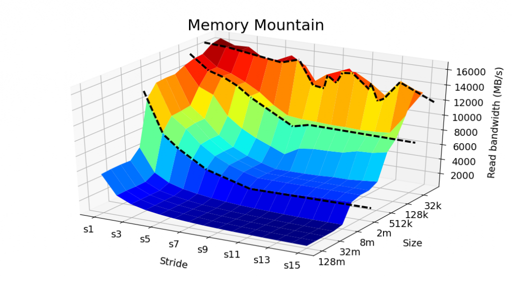
There are many interesting results that can be noted. The black dashed lines show the “size limits” for which we have sharp decreases in the bandwidth for any given stride. For example, as we increase the size from 32 KB, top black dashed line, to 64 KB, the bandwidth dramatically decreases. These limits are indicators of the CPU cache sizes.
The top dashed line corresponds to the L1 cache. It’s the fastest one (thus explaining the greatest read bandwidths), but also very limited in size. Based on the graph, we estimate it to be 32 KB. Next, we have the L2 cache. It’s a bit slower than L1, but larger in size. We estimate it to be 128 KB. Finally, we have the L3 cache. The graph suggests it has a size of 4 MB.
A side-view of the plot helps visualize the cache sizes.
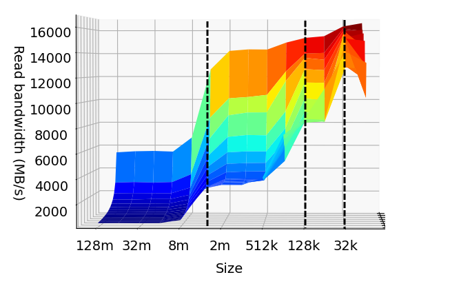
The blue zone with the least read bandwidth, corresponds to the main memory (RAM). The CPU cache is unable to store all of the data for sizes larger than 8 MB (given my system’s hardware). Then, the CPU is required to constantly fetch the information from the main memory. This process is relatively slow and dramatically decreases the read bandwidth.
Spatial locality
A second important result can be seen with the decrease in bandwidth as the stride increases for any given data size. The largest bandwidth, for any size, is obtained through sequential access (stride-1). A more detailed analysis of the effect of spatial locality can be seen in my previous post about array reference performance.
Estimated vs. actual CPU cache sizes
My processor is an Intel Core i5. Its CPU cache specifications correspond pretty well with the results of the memory mountain.
| CPU Cache | Size |
| L1 | 32 KB |
| L2 | 256 KB |
| L3 | 6 MB |
The largest divergence was in the L2 cache size. See that for a size of 256 KB, we get read bandwidths that are in-between a sharp decrease between 128 KB and 512 KB. This could be because the L2 cache is required to store other data besides the array values, being then used beyond its capacity when we test it with an array of 256 KB.
In conclusion
It’s quite amazing to see the effect of low-level hardware on program performance. The most important aspect, however, is what we can learn to write better programs. First, writing programs that process data, as much as possible, in sequential access to exploit spatial locality. And secondly, reduce the size of the working data set that is being processed at a given time to exploit temporal locality.